Wet Dust Collector Design Inputs and Sizing

Wet dust collector design is a chain of inputs, not a vessel selection. The unit cleans only the air that a hood and duct system deliver to it, and that airflow is set at the work point, not on a nameplate. Two shortcuts break projects: sizing a contactor from a cfm figure no capture calculation supports, and comparing quotations built on velocities that mean different things. This guide works the chain in order — capture airflow, dust and gas inputs, type and geometry, water and pressure drop, bleed and solids, and the acceptance inputs to fix before ordering — with one example running grinding dust at 2,000 acfm from hood to sludge. The figures that follow are screening estimates with stated conditions, not a substitute for a vendor design or site test.

Key Takeaways

• Airflow comes from the capture side, not the collector. A wet dust collector design is fixed by hood distance, duct diameter and transport velocity before any vessel dimension is chosen.
• Three velocities carry three different limits. Capture velocity, slot velocity and duct transport velocity are measured in different places and governed by different rules.
• Hood distance decides more than fan capacity. Capture velocity falls by a factor of 10 when the release point moves from one duct diameter to two.
• Transport velocity is a floor. Branch and main minimums exist to keep dust suspended instead of settling into a blocked duct.
• A hood-face figure is not an OSHA number. Manufacturer rules of thumb describe an open hood face, while regulatory limits are tied to duct velocity and distance.

Wet Dust Collector Design Starts at the Capture Point

Capture-side airflow is the first output of a wet dust collector design, and every later number inherits it: contactor diameter, water flow, pressure drop and fan power are functions of the acfm that reaches the unit. The collector creates no capture of its own, so a vessel sized from a nameplate cfm is an unverified assumption with a price attached.

Work backwards from the work point instead. What the process releases, how far the hood sits from that release point, and which duct velocity keeps the dust moving decide the airflow; the collector then treats whatever loading arrives at its inlet. This section fixes those capture-side inputs, because no sizing module further down can correct for an airflow that was never derived.

What the Design Must Output Before Anything Is Sized

Three outputs belong on the drawing before any sizing calculation: the capture velocity required at the work point, the transport velocity that will be held in branch and main, and the system airflow that follows from them, each with its basis written alongside. Capture velocity is the air speed at the release point that pulls dust into the hood. Transport velocity is the speed inside the duct that keeps captured dust suspended on its way to the collector. Slot velocity is the speed through the hood opening itself, and it sets the entry loss the fan has to overcome.

Skipping that step produces a system that is numerically complete and physically empty. A fan curve and a vessel drawing can both be correct while the hood pulls weakly, and OSHA’s ventilation guidance records exactly that pair of outcomes as recurring failures: capture velocity that has declined, and ducts blocked by dust that settled because transport velocity was too low. Airflow is not an independent variable. It is duct area multiplied by velocity, so a 6 in. branch carrying 880 cfm runs at roughly 4,480 fpm, just under the 4,500 fpm branch floor for grinding exhaust.

The basis matters as much as the number. Distance in inches, duct diameter, target velocity and the margin you allow for leakage and later additions all belong on the same sheet as the airflow figure. A supplier receiving only a cfm number cannot check the capture side, and an engineer commissioning the system cannot tell which of the four inputs drifted when measured hood performance falls short of the drawing.

The Three Velocities That Are Not Interchangeable

Capture velocity, slot velocity and duct transport velocity are separate quantities, measured at different places and limited by different rules. Substituting one for another is the most common numerical error in capture-side work, and it happens quietly when a quotation carries a single “velocity” with no location attached to it.

Velocity	What it is	What it controls	Citable limit
Capture velocity (Vc)	The air speed at the release point that draws dust into the hood	Whether dust enters the hood at all, and the airflow the hood needs at its working distance	Simple capture hoods are held at not less than 50 fpm, and the release point should sit no more than 1.5 duct diameters from the hood — with a 6 in. duct that is 9 in. (OSHA ventilation investigation manual)
Slot or hood-face velocity	The average velocity of air through the hood slot or face opening	How evenly air is drawn across a long hood, and the hood entry loss charged to the fan	Minimum slot velocity 2,000 ft/min at a 1/2 in. slot width; entry loss equals 1.0 slot velocity pressure plus 0.5 branch velocity pressure (29 CFR 1910.94(b))
Duct transport velocity	The minimum transport velocity is the minimum velocity that transports particles in a duct with little settling, and it varies with air density and particulate loading	Whether captured dust stays suspended or settles, accumulates and blocks the duct	Recommended minimum 4,500 fpm in the branch and 3,500 fpm in the main for grinding and abrasive cutting exhaust (29 CFR 1910.94(b), Table G-4 context)

Each limit answers a different question, which is why the numbers cannot be traded. The 50 fpm floor describes the air speed a simple hood must produce at a distant release point. The 2,000 ft/min slot figure describes what happens at the hood opening, where a starved slot loses airflow at its far end and the entry loss rises with the square of that velocity. The branch and main figures describe the inside of the duct, where velocity below the minimum turns the duct into a settling chamber. A design can satisfy one of the three and fail on the other two.

Manufacturer sizing pages commonly quote 100-200 fpm measured across the hood face as a rule of thumb. Read that as a vendor convention for simple open hoods, not as a regulatory limit, because it carries no distance and no duct velocity with it, and it is not the figure a compliance inspection looks for. When two quotations arrive with velocities that were measured in different places, the comparison is arithmetic on two different quantities.

Hood Position Before Airflow: The 1.5-Diameter Rule

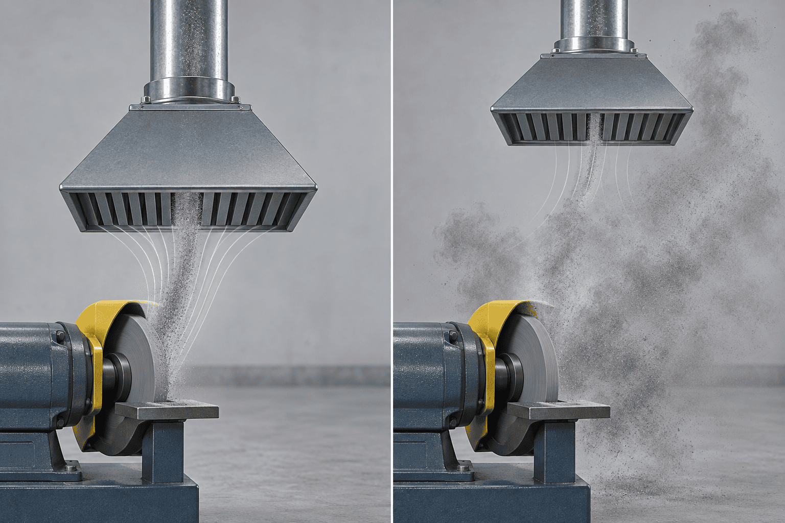
Hood position is fixed before airflow, because the distance between the release point and the hood sets the capture velocity you have to buy. That distance should not exceed 1.5 duct diameters, and the decay behind the rule is steep: with a plain or narrow flanged hood and a duct velocity of 3,000 fpm, capture velocity is about 300 fpm at one duct diameter from the hood, and at two duct diameters it falls by a factor of 10 to about 30 fpm.

Moving a hood from one duct diameter to two is small on a drawing and large in the airflow account. Holding the same capture velocity at the greater distance would take roughly ten times the duct velocity in that hood, and with the duct area fixed that means of the order of ten times the airflow, with fan pressure rising as velocity squared. Reaching such a figure is not a fan selection, it is a different exhaust system, and the cost lands on every hour the unit runs.

Practical limits follow from the same rule. For a 6 in. duct the release point belongs within 9 in. of the hood, and the minimum capture velocity for simple hoods is not less than 50 fpm. Where a process cannot be hooded inside that envelope, enclosure, a slotted hood with slot velocity held at 2,000 ft/min, or a higher airflow with the distance written on the drawing as a stated limitation are the honest options; a larger fan aimed at a remote hood buys airflow that mostly misses the dust.

Set the hood distance, the slot velocity, and the branch and main transport velocities on the drawing before you accept any quoted airflow, and you can decide whether that cfm is a capture-side requirement or a nameplate number.

The Inputs That Decide the Route

Route and geometry are decided by the inputs on the enquiry, not by the equipment menu. Six families carry that decision: particle size distribution and loading; waste gas flow, temperature and humidity; gas velocity and pressure drop; liquid-to-gas ratio; droplet size; and residence time. Each remaining item on the sheet exists to fix one of those six, or to remove an option before the arithmetic starts. Seen alongside the capture-side outputs on the drawing and the acceptance list agreed before the order, these are the same inputs at three stages of resolution: the drawing figures them, the sheet collects them, and the acceptance list fixes them against a test.

Collect the sheet before comparing hardware, and label every entry with its basis: measured, sampled, quoted by a supplier, or assumed. Where a mechanism appears in this section without a cited limit, read it as design reasoning from the physical effect of that input, not as a regulatory value.

Particle Size Distribution and Inlet Loading

Particle size distribution and inlet loading set the route before any geometry is drawn. Distribution decides how much of the dust a contact zone can reach at a given energy input, and loading decides how much material the water circuit has to carry out of the unit and how soon the solids side becomes the limiting part of the design. Neither value predicts performance on its own, which is why the pair travels together.

A distribution arrives as size bands with a mass fraction in each, not as a single mean diameter, and the method behind it belongs on the sheet: sieve, impactor sample or estimate. Keep the fine fraction visible, because the fine end is where a wet contactor loses capture first when energy is held constant, and a mean diameter hides that band.

Inlet loading belongs at the collector inlet with its units and its conditions: grains per cubic foot or milligrams per cubic metre, with gas temperature and moisture stated beside the figure. The same mass at a hotter or wetter condition is a different volumetric duty for the duct and the fan.

Loading reaches into the duct design as well. The minimum transport velocity that keeps particles moving varies with air density and particulate loading, so a denser or heavier stream does not inherit the duct velocity used for a light one, and a velocity copied from a lighter duty is how ducts end up acting as settling chambers. Settling from low transport velocity is one of the two blockage routes that ventilation guidance records, the other being dust wetted by condensation inside the duct.

Dust Properties That Change the Design

Bulk density, stickiness, solubility and abrasiveness change hardware, not the efficiency claim. Each one moves a different downstream parameter, and all four are cheap to establish from a sample or from the process history before the vessel is drawn.

Bulk density separates mass from volume. A storage tank or dewatering step sized on volume behaves differently with dense grinding sludge than with a light fume residue, and the mismatch surfaces as overflow or as haul-off that runs far more often than the plan allowed. Record density at the moisture content of the residue that leaves the unit, because the wet material is what the storage and dewatering step receives.

Hygroscopic and sticky behaviour decides whether the selected transport velocity survives in service. Dust that cakes on contact with moisture bridges hoppers, accumulates in the contact zone and wets inside the duct when vapour condenses there. Where the dust is sticky, cleaning access, sump agitation and a duct route kept above the dew point are design requirements instead of maintenance preferences.

Solubility and abrasiveness pull the specification in opposite directions. Soluble material dissolves into the recirculating water and travels back to the nozzles with the pump loop, so bleed rate and water chemistry carry that load through the whole circuit. Abrasive material wears nozzles, the throat and any wetted bend, so wear allowance and replaceable components belong in the specification, not in the spares list.

Combustibility and reactivity belong on the same sheet as an input variable, because they change downstream requirements: bonding and grounding, detection, isolation, and the way captured residue is handled. Which collection route is safer for a particular combustible metal dust is not settled by any source available here, and this guide does not rank wet against dry for that duty. That decision comes from a site dust hazard analysis, and the comparison itself belongs to a separate article on combustible metal dust.

Gas Temperature, Humidity and Corrosives

Gas conditions set the water balance and the materials, and they are the blank fields that stop a supplier from sizing anything. Waste gas properties are normally given to the vendor so that the system can be sized and the materials chosen, which puts them on the enquiry sheet at the start, not in a later clarification round.

Temperature is a volumetric input before it is anything else. A hot stream is a larger acfm at the collector inlet for the same mass flow, so duct size, fan duty and the contact-zone cross-section all move with it. The same temperature decides how much water evaporates inside the contact zone, and whether the unit must cool the gas before it can saturate it.

Humidity and condensation decide whether the dust arrives dry. Vapour that condenses in the duct wets the particles and builds deposits, the second route to blocked ductwork, so duct routing, insulation and the start-up sequence are design inputs, not field fixes. The same vapour determines what leaves the stack as a visible plume, which some sites have to manage under local expectations.

Corrosives decide materials for every wetted and downstream part: vessel, duct, fan wheel, mist eliminator and pump loop. Acid gases, chlorides and fluorides each act differently on a given material, so the sheet needs the species and their expected concentration, not a general note that the gas is aggressive.

Site Inputs: Water, Power, Space and Discharge

Water, power, plot space and the discharge destination are design inputs, because each one removes options before any calculation runs. A unit with no water quality to feed it, no supply able to start its motors, or no route for its bleed stream is not a design, however well the contact zone calculates.

Water enters the design in four ways: how much is available continuously, how much can be lost to evaporation and bleed, how hard or how loaded it is, and how warm it arrives. Hard or solids-loaded water scales nozzles and the mist eliminator and returns dissolved load to the recirculation tank, pump, filters and valves that the loop depends on, so the water answer belongs with the equipment list.

Power is a starting constraint, not a selection outcome. Available voltage, the largest motor the supply can start, the starting method and the expected duty decide whether a fan and pump combination can be installed at all, and a fan duty calculated before that check is a number with nowhere to land.

Plot space, elevation and maintenance access set the geometry. A vertical contactor needs headroom and rigging space, a horizontal arrangement needs floor area, and both need room to clean the sump, pull the mist eliminator and change nozzles. The discharge destination closes the loop: a drain, an on-site treatment step or a haul-off contract decides how much bleed the site can accept and how the sludge is dewatered, stored and moved. The design ends cleanly only when that route is named.

Input	What it changes downstream	What goes wrong if it is missing
Particle size distribution	Contact type, required energy and the cut diameter the unit has to reach	Efficiency comparisons collapse to a single number with no basis, and the fine fraction is unaccounted for
Inlet particulate loading	Solids load on the water circuit, bleed rate and sludge quantity	Water and residue handling are sized for a cleaner gas than the process produces
Dust bulk density	Hopper, sump and dewatering volumes, and the mass in every sludge figure	Volume-based sizing overflows, or haul-off runs far more often than planned
Hygroscopic and sticky behaviour	Cleaning access, sump agitation, duct routing and the survivable transport velocity	Hoppers bridge and duct deposits build, because the dust was treated as free-flowing
Solubility in water	Bleed rate, water chemistry and the duty on the recirculation loop	Dissolved solids accumulate and return to the nozzles with the pump loop
Abrasiveness	Material and wear allowance for nozzles, throat and wetted bends	Wear parts fail early and the specification carries no replaceable components
Combustibility and reactivity	Bonding and grounding, detection, isolation and residue handling requirements	The safety decision is assumed instead of made; this guide does not rank wet against dry, and that comparison belongs to a separate article
Gas temperature	Volumetric flow, water evaporation, cooling or quench duty and fan selection	The water balance ignores the evaporation load and the fan sees a larger acfm than assumed
Humidity and condensation potential	Duct insulation and routing, start-up sequence and plume expectations	Dust wets inside the duct before it reaches the unit, and the duct becomes the settling point
Corrosives and their concentration	Material selection for vessel, duct, fan wheel, mist eliminator and pump	Materials are chosen on temperature alone, and corrosion shows up as wall thinning and fan imbalance
Available water quantity and quality	Make-up and bleed limits, scaling risk on nozzles and eliminator	The loop is designed for clean water in unlimited supply
Power supply	Largest startable motor, starting method and fan and pump duty	Fan and pump duties are calculated before the supply is checked
Plot space, elevation and access	Contactor orientation, rigging plan and maintenance clearances	Geometry is fixed on paper, and access is discovered during installation
Discharge and effluent destination	Permitted bleed volume, dewatering duty, storage and haul-off	Solids leave the design at the battery limit with no defined route

Bring this sheet to a supplier as one document, and you can decide which parts of the design are still open, instead of discovering them after the purchase order.

Wet Dust Collector Design Basis: Contact Power and Cut Diameter

Efficiency is a result, not a specification, until the basis behind it is written down. A wet dust collector design can be argued in two quantities that survive comparison: the cut diameter, which names the particle size collected at 50% efficiency, and the contacting power, which names the energy per unit of gas the unit spends to reach it. A quotation offering one efficiency percentage, with no particle size distribution and no operating energy attached, describes a measurement whose conditions never reached the buyer.

Three questions settle whether two efficiency figures can be compared at all. What inlet particle size distribution was assumed? At what operating energy was the number measured or modelled? Does the figure describe overall mass removal, or removal in one size band? Answer those and an efficiency number becomes an input to a decision; leave them unanswered and the comparison runs on arithmetic between unrelated quantities.

Why a Removal Efficiency Number Needs a Basis

A removal efficiency figure reports the outcome of a measurement taken against a stated inlet condition and a stated energy input, and neither condition travels with the percentage. The same unit, at the same pressure drop, captures a coarse dust and a fine dust with different results, because the fine fraction is where wet collection loses first. An efficiency number presented without its distribution is a result from somebody else’s dust.

The mass basis hides that difference. Overall removal efficiency is dominated by the size bands carrying most of the mass, so a unit that captures the coarse fraction well reports a high figure while the fine tail passes through. Where the duty is fine dust, the fine tail is the requirement, and a buyer comparing on the headline number has compared nothing that transfers to the site.

Four items turn a claim into a basis: the inlet size distribution the figure was based on, the pressure drop or contacting power at which it applies, whether it is overall mass removal or a band efficiency, and how the number was obtained. Ask for all four and the evaluation becomes technical. A figure without them is a number to be carried as an open item, not a specification to design against.

Cut Diameter Belongs to the Unit, Not to the Dust

Cut diameter is the particle diameter collected at 50% efficiency, and it is a property of the device and its operating conditions, not of the dust’s size range. It is determined from measured collection efficiency and size-distribution data, which is why it moves when the operating point moves: change the energy input or the gas flow and the same hardware carries a different cut diameter.

That distinction is where quotation comparisons break down. A cut diameter printed beside a dust description reads as though the dust owned the number, and the reader then sets it against another unit’s cut diameter measured at a different operating point. The two figures describe two different machines running at two different energy levels, and ranking them means nothing until the operating points match.

Use the cut diameter as a test against your own distribution. Where it sits relative to the mass median of the incoming dust shows how much of that mass the unit can address at the quoted operating point, and the fraction below it is the part that either receives extra energy or leaves with the gas. Read that as screening mathematics with a stated basis, not as a result the unit is obliged to deliver.

Turning the reading into a fractional prediction needs data most sites do not hold on day one. The Calvert method models the penetration of each size band with empirical constants and requires a log-normal particle size distribution as its input. Where the distribution is not log-normal, or measured efficiency data are absent, the fractional prediction is unavailable and the honest route is a test on the actual dust.

Contacting Power and Transfer Units

Contacting power is the energy a scrubber applies per 1,000 acfm of gas, and it is the quantity that ties an efficiency claim to an operating cost. The gas-side term follows pressure drop; the liquid-side term follows liquid inlet pressure and the liquid-to-gas ratio. The gas-side term dominates the total in most wet scrubbers, which is why pressure drop is the figure a proposal should lead with.

The transfer-unit relation converts a fractional removal into a basis for comparing designs. Read it as a ratio, not as a promise: the number of transfer units a given contacting power delivers depends on the scrubber type and on the characteristics of the particulate matter, so one contacting power does not produce the same transfer units in two different designs. The relations below are the set used in the U.S. EPA cost manual chapter for particulate wet scrubbers (wet scrubbers for particulate matter).

Cut diameter. The particle diameter collected at 50% efficiency: a property of the device and its operating conditions, established from measured collection efficiency and size-distribution data.

Calvert cut-diameter method. Pt_j = exp(−A · d_j^B), where Pt_j is the penetration of the j-th particle diameter, d_j that diameter on the aerodynamic size scale in the unit used by the distribution, and A and B empirical constants with B scrubber-specific. It requires a log-normal particle size distribution.

Transfer units. N_t = ln(1/(1 − η)), where N_t is the number of transfer units and η the fractional removal efficiency, entered as 0.95 for 95%. The transfer units a given contacting power delivers depend on scrubber type and on the particulate characteristics.

Contacting power. P_G = 0.157 · ΔP, in hp per 1,000 acfm with ΔP in in. H2O; P_L = 0.583 · p_L · (L/G), in hp per 1,000 acfm with p_L in psi and L/G in gal/ft3. The gas-side term dominates total contacting power in most wet scrubbers.

Used together, the two quantities close the loop on a proposal. Cut diameter states which particle size the unit addresses at its quoted operating point; contacting power states what that point costs in gas-side energy, and through the liquid-side term, in pump energy. Where a proposal supplies a headline efficiency with neither figure, request both and keep the missing values open in the evaluation instead of settling them after the order.

Ask for the cut diameter, the contacting power and the efficiency basis behind any percentage, and you can decide whether two quotations describe the same duty or two different energy levels.

Matching the Collector Type to the Design Inputs

The contactor type follows from the design inputs, and the parameter map is what makes that link checkable. Pressure drop, liquid-to-gas ratio, liquid pressure, gas velocity and cut diameter move as a set by type, so a proposal that names a type without naming those parameters has not answered the duty.

Read the map in the direction of the dust. The fine fraction and the inlet loading decide which class of contactor is capable, and the site inputs decide which capable type can be installed on that plot with that water and power. A type selected first and parameterised afterwards is how a project buys a unit dimensioned for somebody else’s dust.

The Type-to-Parameter Map

The map runs from low-energy to high-energy contactors, and its columns describe one operating regime per type, not five independent adjustments. A spray tower works at a gas velocity of about 10 ft/s and a liquid pressure between 10 and 400 psig, which means the liquid is atomized by nozzle pressure while the gas moves slowly. A venturi operates in the opposite regime: 90-400 ft/s of gas velocity with 0.5-2 psig of liquid pressure, so the gas itself supplies the energy that breaks the liquid into droplets.

Scrubber type	Pressure drop (in. H2O)	L/G (gal/1000 acf)	Liquid pressure (psig)	Gas velocity (ft/s)	Cut diameter (µm)
Spray tower	0.5-3	0.5-20	10-400	10	2-8
Cyclonic	2-10	2-10	10-400	105-140	2-3
Venturi	10-150	2-20	0.5-2	90-400	0.2

Read the ranges as operating parameters for the type, not as guarantees for a particular unit. The liquid pressure column is the source’s own liquid-side parameter in psig and stays labelled that way; it is not the pump head in feet of water that a pump-power relation uses. The cut diameter column is the discarding figure in the table: it states which particle size the type reaches at 50% efficiency, which is the quantity that has to be set against your own distribution.

Published type data puts orders of magnitude behind the table. Spray towers reach as much as 90% removal above 5 µm, 60-80% between 3 and 5 µm, and less than 50% below 3 µm. Cyclonic spray towers reach as high as 95% above 5 µm and 60-75% for submicron particles. Venturi scrubbers range from 70% to 99% above 1 µm and stay above 50% for submicron particles. Those figures carry their size bands and their type; a quotation that borrows one of them without both has borrowed nothing.

Three further relations complete the Calvert method used on the previous page, and all three are type-dependent:

Calvert constants by type. B = 2.0 for venturi, packed bed and tray wet scrubbers; B = 0.67 for cyclonic wet scrubbers, with A and B the empirical constants of the penetration relation.

Cut ratio. Cut ratio = d_cut / d50, where d_cut is the required cut diameter and d50 the mass median aerodynamic diameter.

Overall penetration. Pt_d = integral of Pt_j . m_j, where Pt_d is overall penetration, Pt_j the penetration of the j-th particle diameter size, and m_j the mass fraction of that size.

With the map, the efficiency orders and the constants together, the type decision reduces to three questions: which size band must the unit address, what loading has to pass through the contact zone, and which of the capable types fits the water, power and space available. Answer those and the type is an output of the input sheet, which is where it belongs.

Why Packed Towers Are Not Sized This Way

A packed bed is an absorption device first. Packed towers are most often used for gas adsorption, not for particulate removal, because high particle concentrations build up on the packing and clog the tower. That is the reason a dust duty cannot be sized with the mass-transfer arithmetic of an absorption tower: the height and the transfer units that size a packed bed for a soluble gas describe contact between gas and liquid film, not the capture of particles that are busy filling the same surface.

The constraint is worth stating plainly, because the arithmetic is easy to borrow. Height of a transfer unit and number of transfer units belong to absorption design against a clean gas, and transplanting that sizing onto a dust-laden stream assumes away the mechanism that blocks the bed. Where the duty is dust, the contactors that carry it are argued on cut diameter and on contacting power, and the type parameter map above is the evidence base for that argument.

Where both duties exist, the arrangement follows the same logic. A packed bed earns its place when soluble gas has to be removed, and it then sits downstream of a particulate stage that has already taken the dust out. Sizing the bed first and adding a particulate stage afterwards inverts the duty and returns the clogging problem to the packing.

A proposal that answers a dust duty with a packed tower and a mass-transfer basis has not been sized for the dust. Ask what removes the particulate upstream, and what cut diameter that stage holds at its quoted operating point.

Impingement and Venturi: The Two Workhorses for Dust

Impingement and venturi designs carry most dust duty among wet contactors because both deliver the relative velocity a particle needs to leave the gas stream, and they differ in where that velocity comes from. An impingement-plate design forces the gas through perforated trays or baffles against flowing liquid; a venturi accelerates the gas through a throat and uses the resulting turbulence to atomize the liquid.

The impingement group is built around wetted plates that can be cleaned in service. Gas rises through openings in the trays while liquid flows across them, and the plates are continuously washed by that flow, which is what keeps a wetted surface available for capture. Large particles can plug the perforations, so some designs place impingement baffles upstream of each opening to take the coarse fraction out before the gas reaches it. Published figures for this group put collection efficiency at 97% for particles larger than 5 µm, with submicron removal not effective, gas flows generally between 1,000 and 75,000 scfm, and liquid-to-gas ratios low compared with spray towers and venturis.

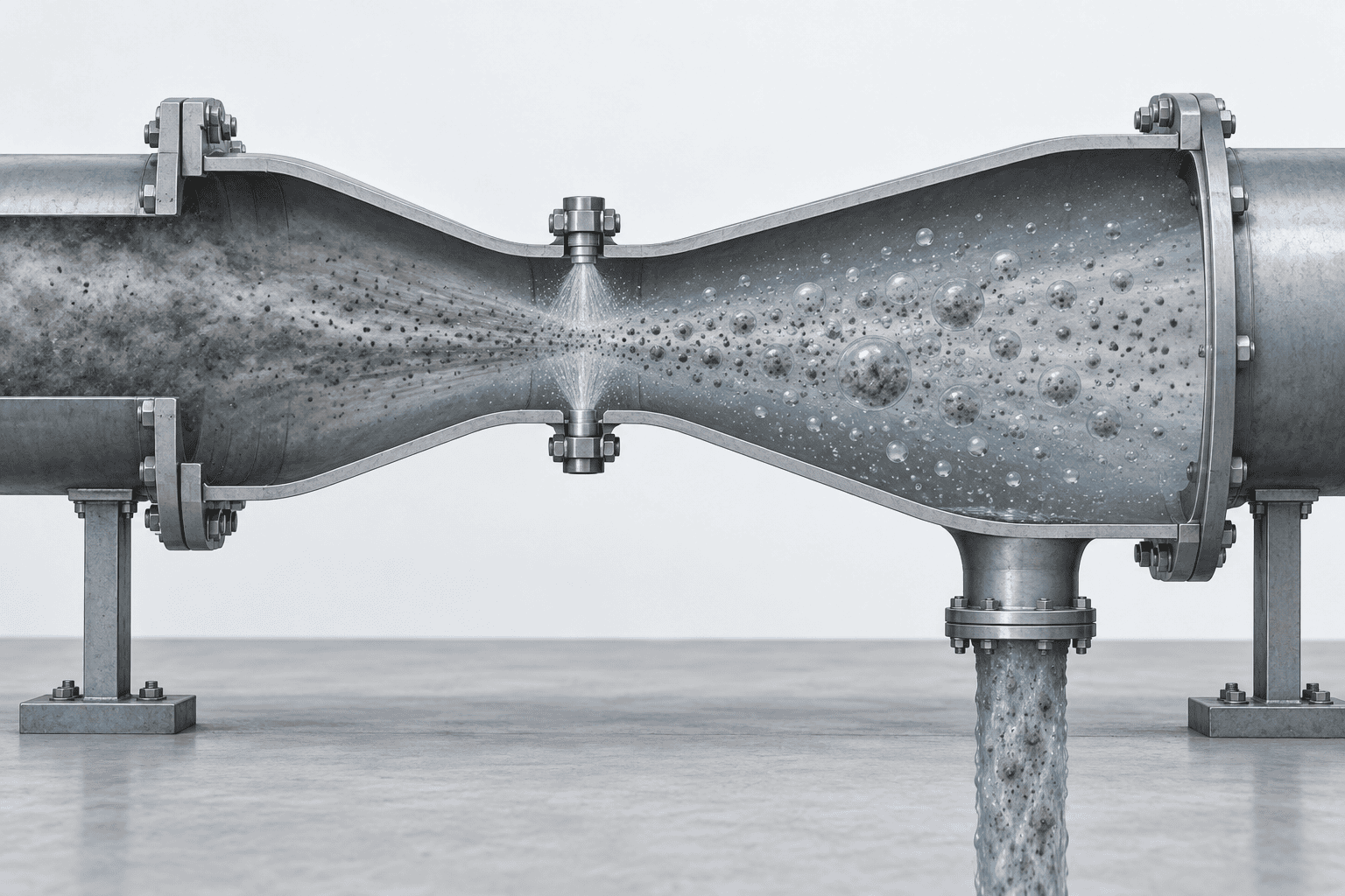
The venturi group is built around the throat. The converging section raises gas velocity and turbulence, liquid is injected just upstream of the throat or directly into it, and the turbulence atomizes the liquid into the droplets that collect particles. The diverging section then decelerates the mixture, which produces further particle-droplet impacts and lets droplets agglomerate before an entrainment section separates them. That is why the venturi holds the smallest cut diameter in the table, and why it buys that reach with pressure drop: published results for the type run from 70% to 99% above 1 µm and stay greater than 50% for submicron particles.

The two groups also separate on maintenance and utilities, which is where the input sheet decides between them. An impingement design carries its liquid at low ratio across wetted plates and is accessible for cleaning tray by tray; a venturi carries its liquid at high velocity through a fixed throat and pays for reach in fan energy, with nozzles and throat as its wear items. Where the dust is coarse and the loading is heavy, the impingement arrangement handles the volume with less energy. Where the fine fraction drives the requirement, the throat is the mechanism that reaches it.

Match the type to the fine fraction and the loading, then check the four parameters a proposal quotes against the map, and you can decide whether a contactor is capable of the duty before the commercial comparison begins.

Sizing the Contact Zone

Contact-zone geometry is a consequence of velocity, and every dimension can be traced back to one. The cross-section follows from the gas volume and the velocity chosen for it, the throat and the diverging section follow from the energy the duty needs and the recovery the fan has to live with, and contact time follows from the length and the velocity at which the gas crosses it. A vessel dimension that cannot be traced to a velocity is a number to query.

The chain set out below is the sizing calculation itself, written so you can reproduce each step on your own airflow and check a quotation against it. Treat the arithmetic as screening geometry with a stated basis: it fixes the order of magnitude and exposes a quoted diameter that has no velocity behind it. It does not replace a vendor design or a test on the dust.

Cross-Sectional Velocity Sets the Diameter

Velocity and volumetric flow together fix the flow area, and the flow area fixes the diameter. That is the whole of the first sizing step: the gas does not care what shape the vessel is, only how much area it has to pass through at the velocity you selected. Written as relations, the step runs A = Q / v with A in square feet, Q in acfm and v in feet per minute, then D = sqrt(4A / pi) with D in feet, multiplied by 12 for inches.

The consequence for comparing quotations is blunt. A quoted vessel or throat diameter with no design velocity attached is not checkable, because the same diameter serves a different flow at every velocity. Ask for the velocity, then reproduce the area and the diameter from it: where the two disagree, the quoted geometry belongs to a different airflow than the one on the enquiry.

As a screening illustration, 2,000 acfm through a 200 ft/s throat needs 2,000 / 12,000 = 0.167 square feet, a diameter of about 0.46 ft, or 5.5 in. Change the target velocity and the diameter moves with it while the airflow stays fixed. The same example inputs are carried into the worked example later in this guide, so the step can be followed here as a screening figure and then again in full, with the same arithmetic and the same checks.

Throat Velocity and the Diverging Section

The highest gas velocity in a venturi occurs at the narrowest cross-section, the throat, and that velocity is generally 150-500 ft/s (45-150 m/s). The pressure loss follows from it: the gas-stream pressure loss across the unit at those throat velocities is 10-80 in. w.c. Throat velocity is the energy dial of the design, and the duty sets it, not preference.

Those ranges sit beside the type-level band of 90-400 ft/s for venturi gas velocity in the previous section, and the two are not the same measurement. The type band describes where venturis are operated overall; the throat figure describes the narrowest cross-section, where the highest velocity in the unit occurs. State which one you mean when a proposal gives a velocity, because a velocity without its location cannot be compared with anything.

The diverging section exists to give that energy back. It is designed to decelerate the gas to 100-50 ft/s (30-15 m/s), where turbulent losses are minimised and the most pressure is recovered, which makes the exit area a sizing step of its own: A_exit = Q / v_exit, taken at the exit velocity, not the throat velocity. A short or abrupt diverging section turns throat velocity into lost pressure the fan pays for on every operating hour.

Read the two areas as a pair when reviewing a drawing. A throat sized for 200 ft/s with an exit sized for the same velocity is a restriction in a pipe, not a venturi: the recovery the diverging section is meant to provide has been designed out of the unit. Give the drawing both velocities and the geometry becomes checkable at a glance.

Contact Time, and the Pressure Drop Ceiling

Contact time is set by length over velocity, and it is shorter than most buyers expect. A venturi with a 1 ft throat length at a velocity of approximately 450 ft/s has a contact time of about 1/450 of a second, roughly 2 milliseconds, and lengthening the throat or the diverging section increases it. Written as a relation, t = L / v, with L in feet and v in feet per second.

The full chain, in the order the geometry is fixed:

Step 1 – Flow area from airflow and velocity. A = Q / v, with A in square feet, Q in acfm and v in feet per minute (multiply a ft/s velocity by 60 first).

Step 2 – Diameter from flow area. D = sqrt(4A / pi), with D in feet; multiply by 12 for inches.

Step 3 – Throat velocity. v_throat generally 150-500 ft/s (45-150 m/s) at the narrowest cross-section, the highest gas velocity in the unit.

Step 4 – Pressure loss from throat velocity. Gas-stream pressure loss across the venturi 10-80 in. w.c. at those throat velocities.

Step 5 – Diverging exit area. A_exit = Q / v_exit, with v_exit 100-50 ft/s (30-15 m/s), where turbulent loss is minimised and the most pressure is recovered.

Step 6 – Contact time. t = L / v, giving about 1/450 s for a 1 ft throat at approximately 450 ft/s; a longer throat and diverging section increase contact time.

Step 7 – Design ceiling. Above 45 in. w.c. of pressure drop, removal efficiency does not increase significantly for conventional venturi designs.

The last step is a check, not a target. Increasing pressure drop above 45 in. w.c. does not significantly increase removal efficiency for conventional venturi designs, so pushing the throat velocity past the loss that corresponds to that ceiling buys fan power without the removal to justify it. The ceiling is stated for conventional designs as published; other arrangements and other duties are different questions.

What the ceiling implies for a design review is the useful part. If the required cut diameter is not reached inside the band the throat can deliver, more velocity is not the answer; the dust data, the contactor type or the arrangement is. Droplet size, liquid-to-gas ratio and contact time carry the rest of the duty, and those inputs are the subject of the next two sections.

Work the chain from airflow and velocity to area, diameter and contact time, and you can decide whether a quoted unit diameter carries a design velocity behind it or is a number with nothing to check it against.

Water and Pressure Drop: The Two Numbers That Set Operating Cost

Two numbers decide what a wet dust collector costs to run: how much water the loop circulates and how much pressure the fan has to overcome. The liquid-to-gas ratio fixes the pump side of the ledger, pressure drop fixes the fan side, and both follow from the geometry and the duty settled in the previous sections. Neither number is a preference, and both are visible on a quotation before any discussion of energy prices begins.

This section converts the contact-zone geometry into a water-and-power account you can reconstruct on your own system. Table 4 collects the quantities, states how each one is fixed, and shows the arithmetic behind the value used in the worked example later in this guide. Cited values keep their published basis, chosen inputs are labelled as examples, and the whole ledger is a screening estimate, not a guaranteed operating point.

L/G Ratio: The Useful Range and the Point of No Return

A venturi performs best with a liquid flow between 7 and 10 gal/1000 ft3, and that band is where a design should sit. Across it, collection efficiency at a constant pressure drop stays fairly constant, which makes the band flat ground, not a slope to climb. Above 10 gal/1000 ft3 the performance does not improve significantly, while liquid consumption and pump work keep rising with every increment.

The mechanism explains the boundary. Adding liquid does not raise the relative velocity between gas and droplets, and once the droplets carry the available surface area, extra flow passes through the contact zone without adding capture. The money still leaves the plant with the bleed stream and through the pump, so past the band the ratio is a cost with no matching return.

Spray towers sit elsewhere on the same scale. Their droplet velocities are low, so they need liquid flows above 20 gal/1000 ft3 to reach comparable contact, which is one reason a spray tower is a poor match for a duty that also carries a tight cut diameter.

Turning the ratio into a flow is the first ledger entry: circulation is the ratio multiplied by the airflow and divided by 1,000. With an example ratio of 8 gal/1000 ft3 on an example airflow of 2,000 acfm, the loop circulates 8 x 2,000 / 1,000 = 16 gpm. That figure is the pump duty, not the nozzle pressure: the liquid-pressure column in the type table is a separate parameter with its own units.

Estimating Pressure Drop From Throat Velocity

Pressure drop across a venturi is estimated from the throat velocity, the saturated gas density and the liquid-to-gas ratio, with the correlation below. The general form leaves the correlation factor to the specific design, which is why a vendor’s own curve remains the authority for a quoted unit.

Calvert pressure drop. dP = 5.4 x 10^-4 x v^2 x rho_g x (L/G), where dP is in inches of water, v the throat velocity in ft/s, rho_g the saturated gas density, and L/G in gal/1000 acf. The general form is dP = k x v^2 x rho_g x (L/G), with k a correlation factor set by the design.

Worked with example inputs: a throat velocity of 200 ft/s, a saturated gas density of about 0.068 lb/ft3, and a ratio of 8 gal/1000 acf. The density here is derived, not measured, by scaling 0.075 lb/ft3 at 70 F to about 120 F on the ideal-gas relation, 0.075 x 530 / 580 = 0.068. The drop then runs 5.4 x 10^-4 x 40,000 x 0.068 x 8 = about 11.8 in. w.c.

Two checks keep that figure honest. It sits inside the venturi band of the type table, and it stays well below the conventional-design ceiling of 45 in. w.c. discussed with the sizing chain, so the energy is doing work the design can use. The mist eliminator adds its own pressure drop of 0.5 to 1.0 in. w.c., and every mist eliminator needs periodic washing to clear particle build-up, which makes that element a maintenance item as well as a pressure term.

Total fan pressure is the sum of the pressure terms: the venturi drop, the eliminator drop, and the losses through hood, duct and connections. Only the first two arrive from the correlations above; the third comes from the layout and needs its own calculation. The ledger uses 4.0 in. w.c. for that item as an example assumption, giving 11.8 + 0.75 + 4.0 = about 16.5 in. w.c. of fan pressure.

Fan Brake Horsepower and Pump Power

Fan power follows pressure and flow, and it is the dominant operating number in most wet dust designs. The relation needs the fan pressure in inches of water, the inlet flow in acfm and the fan efficiency, and it returns brake horsepower at the shaft.

Fan brake horsepower. HP_fan = (dP x Qi) / (6356 x eta_fan), where dP is fan pressure in in. w.c., Qi the inlet flow in acfm, and eta_fan the fan efficiency.

With the example ledger, 16.5 in. w.c. of fan pressure on 2,000 acfm and an example fan efficiency of 0.65 gives (16.5 x 2,000) / (6356 x 0.65) = about 8 hp. Both the efficiency and the 10% airflow margin behind the 16.5 in. w.c. are example inputs; a different fan efficiency moves the result in proportion, which is why a proposal should state the efficiency it assumed.

Pump power follows the same logic with one trap worth naming. The pump relation takes head in feet of water, while the fan relation takes pressure in inches: the two are not interchangeable, and the liquid-pressure column of the type table is neither of them.

Pump brake horsepower. HP_pump = (dP_pump x Qi x gamma x (L/G) / 1000) / (3952.6 x eta_pump), where dP_pump is in feet w.c., L/G in gal/1000 ft3, gamma the specific gravity of the scrubbing liquid, and eta_pump the pump efficiency.

With 40 ft w.c. of example pump head, an example efficiency of 0.6, a specific gravity of 1.0 and the same ratio of 8, the pump works out at (40 x 2,000 x 1.0 x 0.008) / (3952.6 x 0.6) = about 0.3 hp. The comparison is the point of the pair: the fan carries the design’s energy bill, and the pump loop is a smaller but continuous draw whose size is set by the ratio selected in the first part of this section.

Quantity	How it is fixed	Value or basis
L/G ratio	The venturi optimum band; above the band adds cost without performance	7-10 gal/1000 ft3 optimum for a venturi; the example uses 8 (example input). Spray towers need above 20 gal/1000 ft3
Circulating water flow	L/G x airflow / 1,000	Example: 8 x 2,000 / 1,000 = 16 gpm (derived from an example ratio)
Pressure drop across the venturi	Calvert relation from throat velocity, saturated gas density and L/G	Example: 5.4 x 10^-4 x 200^2 x 0.068 x 8 = about 11.8 in. w.c. (derived; density derived from 0.075 lb/ft3 at 70 F scaled to about 120 F)
Mist-eliminator pressure drop	Published range for mist eliminators, with periodic washing required	0.5-1.0 in. w.c.; the example uses the mid-value 0.75 (example value inside a cited range)
Hood, duct and connection losses	Layout and fittings; requires its own calculation	4.0 in. w.c. assumed for the example (example input)
Total fan pressure	Sum of the pressure terms above	Example: 11.8 + 0.75 + 4.0 = about 16.5 in. w.c. (derived)
Fan brake horsepower	HP_fan = (dP x Qi) / (6356 x eta_fan), dP in in. w.c.	Example: (16.5 x 2,000) / (6356 x 0.65) = about 8 hp (derived; 0.65 fan efficiency is an example input)
Pump brake horsepower	HP_pump = (dP_pump x Qi x gamma x (L/G)/1000) / (3952.6 x eta_pump), dP_pump in feet w.c.	Example: (40 x 2,000 x 1.0 x 0.008) / (3952.6 x 0.6) = about 0.3 hp (derived; 40 ft head and 0.6 efficiency are example inputs)
Bleed fraction	Set by the solids concentration the loop can carry, held between 20 and 30 percent by weight	The example holds the bleed at 25 percent solids (example value inside a cited band)

Read the ledger as an operating account, not a specification. The cited values state where the design should sit; the example values show the arithmetic; and the quantities the ledger cannot supply, such as the layout losses and the actual pump head, remain open items until the site geometry is fixed.

Fix the ratio inside the optimum band and read the pressure drop from the throat velocity, and you can decide which of the two running costs a proposed design change is moving, and by how much of the ledger.

Mist Elimination and What It Adds to the Design

Mist elimination is a design stage in its own right, not an accessory fitted once the contact zone is finished. Every droplet that leaves the contact zone carries captured dust with it, so the separator decides whether the material just removed stays removed or travels on to the fan, the ductwork and the stack. A design that treats the eliminator as an accessory gives back part of what it has already paid for.

This section covers the two things the water-and-pressure ledger could not: what the eliminator exists to protect in the system, and the washing provisions that belong on the drawing as design requirements. The eliminator’s own pressure drop and the fact that all mist eliminators need periodic washing were settled with the ledger, and neither is re-derived below.

Mist Eliminator Duty and Its Pressure Drop

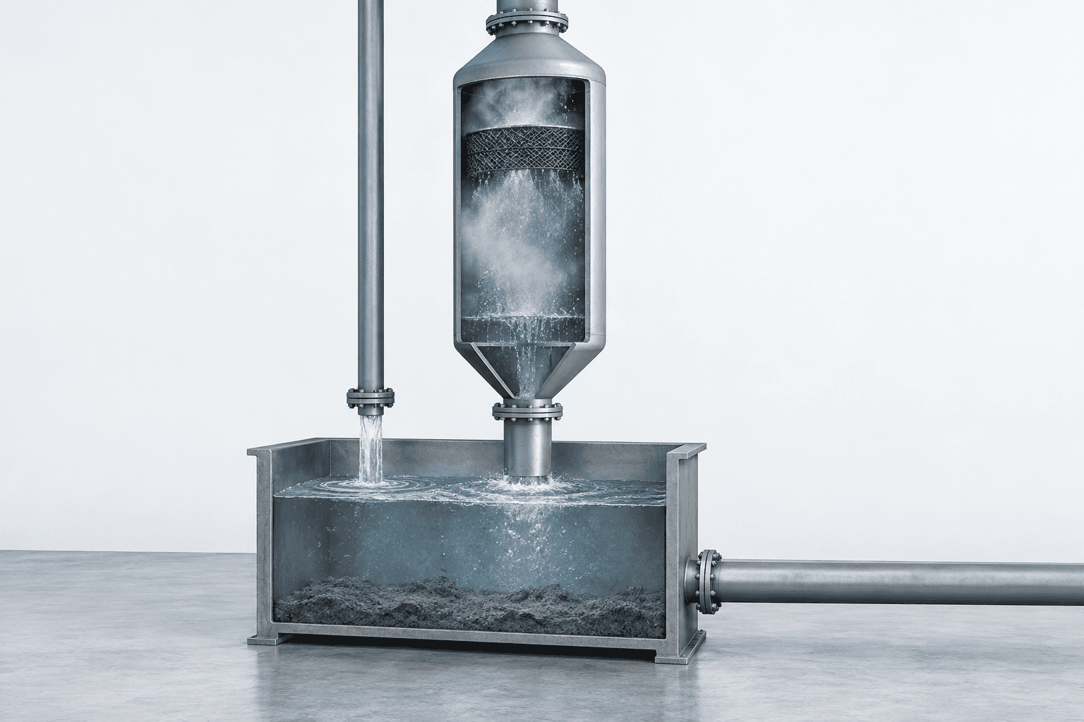
Droplets that remain entrained in the gas stream after the contact zone are generally removed with a mist eliminator, which makes it the last stage that keeps captured material out of everything downstream. In a venturi system a separator, often a cyclone, plus a mist eliminator sit between the contact zone and the clean gas outlet. The collection chamber that hosts the eliminator can be a simple tower, a baffled tower or a cyclone; the baffled and cyclonic forms separate more liquid and dust, using impaction alongside gravity, and they charge for that improvement in pressure drop.

The eliminator also holds a defined place in the system component list a venturi specification should follow: liquid storage and delivery, liquid injection, the venturi throat section, the collection chamber with a mist eliminator, waste liquid collection and disposal, instrumentation and controls, and auxiliary equipment. Read that list against a proposal and the eliminator is easy to locate. An item missing from the list is a duty with no owner.

The design has to deliver three things from that position. Separated droplets must coalesce and drain back to the sump instead of re-entraining, which is a matter of how the surface sheds liquid. The elimination surface must suit the gas velocity it faces, because a surface overloaded at its face re-entrains the liquid it has just separated. And the dust carried in those droplets must be out of the gas before the outlet, since it is the same material the contact zone was built to capture.

The duty has a separation figure attached to it, and its scope matters as much as its value. Mist eliminators remove between 90% and 99% of the liquid droplets from the waste gas stream. That is a droplet-separation figure and nothing more: it says nothing about particulate removal, so it cannot be read as a dust-removal efficiency for the unit. The dust leaves the gas earlier, in the contact zone, and the eliminator is what stops the droplets that carry it from travelling on.

Two design families cover most of the duty, and their weakness differs. Droplets collect and coalesce on chevron blades or on a mesh pad, and once they are large enough they fall by gravity or capillary action. Mesh pads can be clogged by particulate, which is why chevron designs are more frequently applied to dust service. Whichever form is offered, the material decision follows the wetted service: waste gas properties are given to the vendor to size the system and to choose materials, and the eliminator sits in that same wet, corrosive stream as the vessel and the duct.

Carry-over is what the design is protecting against, and the consequences land in three places. Deposits build in the ductwork downstream, where they add weight and, in time, restrict the flow the fan was sized to move. They build on the fan itself, where imbalance costs bearings and cleaning time. And captured dust can leave with the outlet gas, which returns part of the removal duty to the room or the stack. None of those outcomes announces itself as a separator problem; each appears as a duct, fan or emission complaint months after commissioning.

Washing as a Design Input

Washing is a design input because every mist eliminator requires periodic washing to remove particle build-up. The requirement is not an intention expressed in an operating manual; it is a provision the drawing has to supply, in the same way that the throat and the sump are supplied. A design that leaves washing to the operator has left a duty with no equipment behind it.

Four provisions belong in that package. The eliminator needs access to be washed and, when necessary, removed, which means a hatch, clearance and lifting provision, not a sealed chamber. It needs a wash arrangement, whether fixed headers, manual wash points or flooding, with a supply that reaches both faces where the build-up collects. It needs wash water of a quality that does not scale the elimination surface, which puts the site’s water analysis back into the design instead of the maintenance file. And it needs materials chosen for a wet, loaded service, not for the clean-gas side of the unit.

The consequence of designing without them is a permanent cost, not a deferred task. A blinded or scaled eliminator raises its own pressure drop above the clean figure the ledger carries and separates less effectively, so the site pays twice: in fan energy on every operating hour, and in the carry-over risk that returns dust to the duct, the fan and the outlet. No figure is quoted here for a fouled or washed element, because the published range describes a clean surface, and the drift from it depends on the dust.

That gives a design review a short question to ask of any proposal: where does the wash water enter and leave, how is the element reached, what water quality was assumed, and what material is the element made from. A proposal that lists a mist eliminator without those answers has left the owner with the operating problem.

Place the eliminator in the system component list and specify its washing provisions as design requirements, and you can decide whether a proposal has treated carry-over as a duty or as an accessory.

The Sludge and Bleed Ledger as Design Inputs

Everything the contact zone captures leaves the unit as a stream that has to be defined, sampled and sent somewhere. Spent scrubbing liquid drains from the bottom of the collection chamber to the recirculation tank, and a portion of it is bled from the system to hold the solids concentration inside a limit; what leaves on that bleed line is a slurry with a high solids content, and in some applications it may contain hazardous material. The design task is to size that stream and to name its destination.

This section builds the ledger the same way the water and power account was built: a cited rule where one exists, a reproducible example where the arithmetic has to be shown, and an honest marker where the design stops and a site decision begins. The route comparison against dry collection sits in a companion article, and the waste determination sits with the site.

Bleed Rate and Solids Concentration

Bleed rate is set by the solids concentration the recirculating loop can carry, and for a venturi system that concentration is limited to between 20% and 30% by weight. The bleed is the control on that limit: liquid drains from the collection chamber to the recirculation tank, a portion is drawn off, and make-up water replaces it so the loop keeps working with a liquid whose solids content stays inside the band.

The mechanism explains why the bleed cannot be treated as a disposal detail. A loop that never sheds solids concentrates them every hour it runs, and the liquid eventually stops behaving like the liquid the nozzles and the contact zone were selected around. Solids also settle wherever velocity falls, so an over-concentrated loop loads the sump, the filters and the spray path at the same time.

The bleed is small against the circulation, which is what makes steady control possible. In the example ledger the loop circulates 16 gpm and the bleed leaves at roughly 0.2 gpm, about one percent of the circulating flow. A small, continuous bleed holds a steady concentration; a large intermittent one swings the loop between dilute and loaded, and each swing shows up as a change in spray behaviour and as a number nobody is watching.

Loading pushes the bleed rate up, and the direction of the consequence is fixed: a higher particulate loading in the gas requires a higher bleed rate, which produces a greater volume of liquid waste and higher disposal costs. That relationship is the reason the inlet loading from the input sheet is a water-side design input and not only a capture-side one.

Estimating the Sludge Mass

The solids entering the liquid are estimated from the inlet loading, the gas flow and the design capture, using the mass-flow relation m_PM = eta x L_PM x Qi, where eta is the fractional collection efficiency, L_PM the particulate loading at the inlet and Qi the inlet gas flow. The result is a mass rate of particulate into the scrubber liquid, and it is the quantity every downstream item in the sludge ledger is built from.

Worked with the example inputs: an inlet loading of 2 gr/ft3 on 2,000 acfm gives 4,000 gr/min, which is about 34 lb/h once grains are converted at 7,000 grains to the pound. Applying the example design capture of 95% leaves about 33 lb/h of solids to be carried out of the system in the liquid. Both figures are example values, and the conversion is the only arithmetic needed to reach them.

Holding the bleed at 25% solids by weight turns that mass into a slurry rate: about 33 lb/h of solids behind a bleed held at a quarter solids gives roughly 130 lb/h of slurry, with the water fraction at about 98 lb/h and the rounding spread across the two figures. The water fraction is the part an operator sees, and it is close to 0.2 gpm, which is why the stream is small in volume and difficult to handle by volume alone.

The linearity is the useful property of the relation. Sludge mass scales with loading and with the capture applied to it, so doubling the loading doubles both the solids and the bleed, and a change of capture target moves the solids rate in proportion. Storage, dewatering and haul-off intervals are all sized from that mass rate, which is why the inlet loading deserves a measured value instead of an estimate copied from a similar process.

Dewatering, Discharge and Where This Design Stops

Dewatering and discharge are where the scrubber design hands over to the site. The dewatering duty follows the solids mass rate, the storage volume follows the bleed rate and the interval between collections, and the destination is a site decision: a drain, an on-site treatment step or a haul-off arrangement. None of the three is settled by the contact-zone geometry, and all three belong on the drawing before the order.

The design’s own obligation is narrower than the disposal question, and worth stating in those terms. What the design can deliver is a defined and samplable interface: a bleed stream with a stated flow and a stated solids concentration, a sample point that represents that stream, and a named destination for what leaves it. Whether the captured material is a hazardous waste is a separate determination, made against the applicable waste rules and the site’s own analysis of the residue, and this page does not classify any residue, does not rank disposal routes and does not promise a disposal outcome. In some applications the effluent may contain hazardous material, which is exactly why the sample point and the destination are design items and not an afterthought.

Two items stay open on purpose. The moisture of the dewatered residue follows the dewatering equipment selected, not the scrubber, and the storage interval follows the site’s logistics. Carrying both as named open items keeps the ledger honest, and it gives the site the two figures it needs to finish the job.

Input	How it is fixed	Value or basis
Bleed rate and solids concentration limit	The bleed is set to hold the loop’s solids content inside the published band	Band 20% to 30% by weight for a venturi system (cited); the example holds 25% (example value inside a cited band)
Particulate mass flow into the liquid	m_PM = eta x L_PM x Qi, with eta the fractional capture, L_PM the inlet loading and Qi the inlet gas flow	Example: 2 gr/ft3 on 2,000 acfm = 4,000 gr/min = about 34 lb/h (derived)
Captured solids mass rate	The inlet mass flow multiplied by the design capture	Example: 95% of about 34 lb/h = about 33 lb/h (derived; the 95% capture is an example target)
Slurry mass rate	Captured solids divided by the solids fraction held in the bleed	Example: about 33 lb/h / 0.25 = about 130 lb/h (derived)
Water fraction of the bleed	Slurry mass less the solids mass	Example: about 98 lb/h of water in the bleed, close to 0.2 gpm (derived)
Bleed against circulation	The bleed flow compared with the loop circulation from the water and power ledger	Example: about 0.2 gpm against 16 gpm, roughly one percent (derived)
Sludge moisture	Fixed by the dewatering step selected, not by the scrubber	Open item: the example leaves cake moisture to the dewatering selection (design reasoning)
Dewatering duty	Set by the solids mass rate and the cake moisture chosen	Example: about 33 lb/h of dry solids sets the duty (derived, with the equipment rating still open)
Storage volume	Set by the bleed rate, the solids settling behaviour and the interval between collections	Example: sized from about 130 lb/h of slurry over an interval chosen by the site (derived, interval open)
Discharge destination	A site decision among drain, on-site treatment or haul-off	Must be named before the design closes (design requirement)

Fix the bleed at a stated solids concentration and size the discharge route from the solids mass rate, and you can decide what leaves the design as a defined stream instead of an open item.

Acceptance: What to Fix Before the Purchase Order

Acceptance is where a design becomes enforceable, and it is fixed before the order, not after commissioning. Every performance figure depends on the conditions it was measured at, so the acceptance section of an enquiry is a list of inputs that both parties agree to hold constant: the dust data, the gas conditions, the operating point, and the way a test will be run. Items left open here are argued about later, when the unit is installed and nobody can reconstruct what was assumed.

This section is the article’s checklist, and it holds to one rule. No guarantee value, tolerance, permitted deviation or test duration appears below, because the sources behind this guide carry none, and a number invented here would be worse than an item left to the parties. What follows names the inputs that have to be agreed and says why each one becomes unarguable once the equipment is built.

Test Conditions and Tolerances

A test condition has to state the same parameters the design was built on: the particle size distribution and loading, the waste gas flow, temperature and humidity, gas velocity and pressure drop, the liquid-to-gas ratio, droplet size and residence time. Those are the design parameters of the unit, and a test that fixes only some of them measures something without measuring the duty the equipment was bought for.

The cut diameter is the reason the operating point cannot be left implicit. Cut diameter is a characteristic of the device and its operating conditions, established experimentally from measured collection efficiency and size-distribution data, so the same hardware at a different flow, pressure drop or liquid ratio becomes a different unit on paper. A performance figure that arrives without its operating point cannot be compared with anything, including the same supplier’s earlier offer.

Waste gas properties are normally given to the vendor so that the system can be sized and the materials chosen, which means the input sheet already exists before the test is discussed. Tied to a measured operating point, that sheet becomes the test condition list; the work is to add the operating point and the measurement plan, not to build a second document.

The measurement plan is part of the conditions, not an administrative detail. Duct velocity can be measured directly with velometers and anemometers, or indirectly with manometers and pitot tubes through duct velocity pressure. Airflow in industrial ducts is almost always turbulent with a thin non-moving boundary layer at the duct surface, and because velocity varies with distance from that edge, a single measurement may not be sufficient. Where the probes go, how many traverse points are used and which duct is sampled decide whether the result describes the system. The same ventilation guidance records reduced capture velocity and plugged ducts as the common failure signatures a test is meant to catch.

Tolerances belong on the same list, as agreed items and not as defaults. Whether the agreed airflow may drift during a test, and by how much, is a figure the parties have to fix in the acceptance section; the same applies to how ambient conditions and normal process variation are treated. No figure is offered here for any of them, and that absence is deliberate: an assumption presented as a standard is how acceptance disputes start.

Guarantees and Their Boundaries

A guarantee is a claim attached to conditions, and its boundary matters as much as its level. What the unit will do at the agreed inlet conditions and the agreed operating point can be guaranteed; what it will do on a different dust, a different loading or a different gas temperature is a question about a different unit. The enquiry should therefore fix both sides of the line: the conditions inside the guarantee and the conditions outside it.

The type’s own parameter ranges are what a claim should be traceable to. Pressure drop, liquid-to-gas ratio, gas velocity and cut diameter are published as ranges for each contactor type, so a guarantee that sits outside those ranges is asking a type to do something it is not described as doing. Ask the supplier to place the offer inside the range and to state the operating point that the guarantee attaches to.

A workable guarantee names its own basis. It states the inlet conditions it applies to, the pressure drop or contacting power it attaches to, the cut diameter or size band it is claimed against, the measurement methods and sampling locations, and who runs the test. It also states what happens when the agreed conditions are not met on the day, so that a shortfall in the test conditions is not silently converted into a shortfall in the equipment. This guide takes no position on the numbers those items should carry.

The boundary should close the battery limit as well. The bleed flow and solids concentration, the sample point that represents them and the destination for what leaves were fixed in the sludge ledger, and they belong in the guarantee discussion for the same reason the air side does: an interface nobody guaranteed is an interface nobody owns. Whether the captured material is a hazardous waste remains a site determination made against the applicable waste rules, and it is not part of the equipment guarantee.

When a Pilot Test Is the Only Honest Answer

Where the dust data are unavailable, or the distribution does not meet the requirement of the prediction method, an honest number cannot be produced by calculation and a pilot test is the only defensible route to one. The Calvert method models penetration against a log-normal particle size distribution; where that condition fails, or where measured efficiency data are absent, the fractional prediction is simply unavailable.

A pilot test is only useful if it carries the same discipline as a full-scale test. It needs the condition list from the first part of this section, a defined sampling point and analytical method, an agreed operating point, and a stated basis for translating what happens in the test unit to the full-scale design. Without that last item the result describes a test rig, and it cannot be compared with the correlated ranges the proposal is built on.

The honest alternative exists and is worth using. Where even a pilot is out of reach, the enquiry can say so and write the acceptance against the agreed conditions and the agreed operating point instead of against an outcome, which keeps every party on defensible ground. Nothing in this section is a sales step: a pilot test is the route a design takes when the data needed to argue it are missing.

Order matters more than wording. Fix the inlet and gas conditions, agree the operating point and the test method, define the guarantee boundary, and only then compare commercial offers. Every one of those items is cheaper to settle before the order than after the equipment is on the ground.

Input to fix	Why it has to be fixed before the order	What to state
Particle size distribution basis	The cut diameter claim is read against this distribution	Size bands with mass fractions, the method behind them (sieve, impactor or estimate), and whether the distribution meets the log-normal requirement
Inlet loading and its basis	Loads the sludge ledger and the capture claim at the same time	The loading with its units, how it was established, and whether the figure is a peak or an average
Design gas flow and its basis	Fixes the contact-zone geometry and the fan duty	The flow, the capture-side basis behind it (stations, hoods, velocity floors, margin), and how drift is to be treated as an agreed item
Gas temperature and moisture	Drives the volumetric duty, the evaporation load and the material choice	The range, the saturation assumption, and where the figures come from
Pressure drop or contacting power	Without the operating point the claim cannot be checked	The value the guarantee attaches to, and which of the two governs the agreement
Cut diameter or size band claimed	The claim has to name the particle size it refers to	The cut diameter or size band claimed, and the published type range it sits inside
Performance test measurement methods	The method decides whether the result means anything	The instruments and the approach (direct velocity instruments or a pitot traverse), plus the dust sampling and analytical methods
Sampling locations	Velocity varies across the duct, so one reading may not be sufficient	The duct, the traverse points, and the inlet and outlet sample positions
Guarantee boundary	A claim without a boundary is a claim to nothing	The conditions inside it, the conditions outside it, the party who runs the test, and what a condition shortfall does to the guarantee
Residue and discharge interface	The design ends at the battery limit named in the sludge ledger	The bleed flow and solids concentration, the sample point, and the named destination
Tolerances and test duration	The sources carry no figures for these, so the parties have to agree them	State them as agreed items written into the acceptance section, not as defaults assumed by one side

Fix the condition list, the operating point and the measurement method before the order, and you can decide what is being guaranteed, on what basis, and which parts of the design are still assumptions.

Where the Design Usually Goes Wrong

Most wet dust collector failures are not equipment faults; they are design inputs that were left open and were later discovered by the plant. The failures below share a shape: a value was assumed, copied or skipped, and the consequence appeared months afterwards as a capture complaint, a blocked duct, a fan that will not settle or a slurry with nowhere to go. Read backwards, each failure names the input that would have prevented it and the section of this guide that fixes it.

The table is the back-reference index for everything above. Where a failure appears, the correction is rarely a component upgrade; it is a value that should have been on the drawing before the order.

Failure Modes and the Input That Prevents Them

Failure at the unit	The design input that prevents it	Where that input was fixed
A system airflow with no capture basis	A system airflow derived from the hood, the duct velocity and a stated margin	The capture side: airflow is duct area multiplied by velocity, not a nameplate figure
Weak capture at the work point	Hood distance held inside the limit, with the minimum capture velocity set at the source	The capture side: the source sits no more than 1.5 duct diameters from the hood, and the minimum capture velocity for simple hoods is not less than 50 fpm
Duct blockage from settling	A transport velocity set for the dust being carried, not copied from a lighter duty	The capture side: the minimum transport velocity varies with air density and particulate loading, so a heavier stream does not inherit the same duct velocity
Duct blockage from condensation	Dust kept above its dew point, with duct routing, insulation and start-up sequence designed for it	The input sheet (gas temperature and humidity) and the capture side’s second blockage route
Fan energy spent for no removal	A throat velocity inside the range the type can use	The sizing chain: above 45 in. w.c. of pressure drop, removal efficiency does not increase significantly for conventional venturi designs
Water cost without contact	The liquid-to-gas ratio held inside the optimum band	The water ledger: the optimum is 7 to 10 gal/1000 ft3, and above 10 the performance does not improve significantly while liquid and pump usage keep rising
Packing fouled by dust	Contact type chosen for particulate duty, with a particulate stage upstream of any packing	The type map: packed towers are most often used for gas adsorption, because high particle concentrations build up on the packing and clog the tower
Eliminator blinded or scaled	Washing provisions specified as design requirements, not implied	Mist elimination: every mist eliminator requires periodic washing, and access, wash arrangement, water quality and materials have to be designed in
An efficiency figure with no basis	The operating point and the size basis stated with the number	The design basis: cut diameter is a characteristic of the device and its operating conditions
A slurry stream nobody sized	A bleed rate set from the inlet loading, with the discharge interface named	The sludge ledger: a higher particulate loading requires a higher bleed rate, and the bleed is held against the solids concentration limit
A design argued on dust data that does not exist	A measured distribution, or a pilot test where prediction is unavailable	The acceptance list: the Calvert method requires a log-normal particle size distribution

The clustering is the useful part of the pattern. Capture-side inputs account for the first four failures, and they are the ones that surface in service earliest, because the room complains before the duct blocks. Water-side inputs account for most of the rest: a ratio set above the band, a packing that fills with dust, an eliminator that blinds, and a bleed that cannot keep pace with the loading.

Two of those failures look alike and are not. Duct blockage from settling happens when the velocity is too low for the dust being carried, and it grows from the bottom of the duct. Blockage from condensation happens when vapour condenses inside the duct and wets the particles, and it grows wherever the gas first falls below its dew point. One is a velocity input and the other is a temperature and humidity input, so a design that fixes one while leaving the other open has half a duct design.

The last three failures are commercial in appearance and technical underneath. A diameter quoted without a velocity, an efficiency figure without an operating point, and an acceptance section without agreed conditions all pass an internal review, and each one fails at the first serious comparison between offers or at the performance test. They are the reason the back-references above point at conversations and not at parts.

What the Calculation Cannot Replace

The chain in this guide is screening geometry and hydraulics with a stated basis, and it does not replace four things: a test on the actual dust, a vendor’s own design and guarantee, a professional review of the installation, and the site’s waste and discharge determinations. Those four cover the ground the correlations cannot reach, and each has an owner other than this page.

What the arithmetic does is narrower and still valuable. It positions the design, exposes assumptions that would otherwise stay invisible, and gives you the questions to put to a proposal. A throat diameter that reproduces from airflow and velocity, or a sludge rate that follows from loading and capture, tells you that the offer was built the same way the duty was.

Four items stay open by design in this guide: the layout losses through hood, duct and connections, the actual pump head, the moisture of the dewatered residue, and the interval between collections. Leaving them open is not the same as leaving them unmentioned. An open item is named, has an owner at the next stage and travels into the acceptance discussion; an omission is discovered by the operator, usually on a weekend.

That distinction is worth applying to any proposal you receive. A design that lists its open items is more useful than one that appears complete, because the complete-looking version has hidden its assumptions until commissioning, which is the latest and most expensive moment to meet them.

Check the failure list against your own drawing, and you can decide which inputs are still open before they become complaints about capture, blocked ducts, energy or residue.

Worked Example: Metal Grinding Dust at 2,000 acfm

The chain below runs the whole method on one duty: two metal grinding stations exhausting through a wet venturi, from the hood to the acceptance list. Every value is labelled as cited from a source, derived by arithmetic, or chosen as an example input, so you can rebuild the steps with your own numbers and see exactly which ones move.

The case: two grinding stations with wheels between 24 and 30 in. in diameter and 5 in. wide. The airflow is not taken from a collector nameplate; it comes out of the operating table and the velocity floors, and that is the first thing the example demonstrates. The example values are the author’s choices for this case, not recommendations, and none of the results is a guaranteed performance figure.

Steps 1-2: From the Hood to the System Airflow

Step 1 sets the minimum exhaust volume per station. For grinding wheels in that size range, the operating table gives a minimum of 880 cfm per station, and that value is cited, not chosen. Two stations, each on its own branch, is the layout the example works with.

Step 2 checks the branch against the velocity floor, and this is where the table figure stops being a design airflow. A 6 in. round branch has an area of about 0.196 ft2, so 880 cfm through it runs at 880 / 0.196 = about 4,482 fpm. The recommended minimum duct velocity is 4,500 fpm in the branch, so the table value lands just under the floor. The airflow moves instead of the floor: at 900 cfm per station the same branch carries about 4,584 fpm, above the minimum.

The system airflow then follows from the capture side. Two stations at 900 cfm give 1,800 cfm, and a margin of 10% for leakage and later additions, which is an example input, gives 1,980 cfm, carried through the rest of the chain as 2,000 acfm. The main duct is checked against the cited floor of 3,500 fpm when it is sized; that check belongs to the layout, not to the collector.

Steps 3-4: Type, Throat Velocity and Contact Time

Step 3 selects the contactor. Grinding dust carries a fine fraction, so the example takes a low-energy venturi and justifies it against the type map: the venturi row holds the smallest cut diameter of the three types, its pressure drop band runs from 10 to 150 in. w.c., and its gas velocity band runs from 90 to 400 ft/s. The throat velocity chosen for the example is 200 ft/s, inside the cited throat band of 150 to 500 ft/s, and it is an example input, not a requirement.

The throat geometry follows from that velocity and the system airflow. At 2,000 acfm the flow is 2,000 / 60 = 33.3 cubic feet per second, so the throat area is 33.3 / 200 = 0.167 ft2, and the equivalent diameter is sqrt(4 x 0.167 / pi) = 0.46 ft, or about 5.5 in. Those two figures are derived; change the velocity and both move.

Step 4 gives the contact time. A throat 1 ft long with gas moving at 200 ft/s passes the gas through in 1 / 200 = 0.005 seconds, about 5 milliseconds. The published reference point for the type is a 1 ft throat at approximately 450 ft/s, which gives about 1/450 of a second; the example runs longer because its throat velocity is lower, and that difference is the trade against pressure drop that the next step quantifies.

Steps 5-6: Water, Pressure Drop and Power

Step 5 fixes the water. The example takes a liquid-to-gas ratio of 8 gal/1000 acf, an example input sitting inside the cited optimum band of 7 to 10 gal/1000 ft3, where collection efficiency stays fairly constant at a constant pressure drop. Circulation follows by multiplication: 8 x 2,000 / 1,000 = 16 gpm. That flow is the pump duty; the liquid-pressure column in the type table is a different parameter with different units.

Step 6 estimates the pressure drop, and it starts with gas density. Taking 0.075 lb/ft3 at 70 F and scaling to about 120 F on the ideal-gas relation gives 0.075 x 530 / 580 = 0.068 lb/ft3, a derived value for saturated gas. The Calvert relation then gives the drop: 5.4 x 10^-4 x 200^2 x 0.068 x 8 = about 11.8 in. w.c. Two checks apply to that result: it sits inside the cited venturi band of 10 to 150 in. w.c., and it stays well below the 45 in. w.c. level above which conventional venturi designs do not gain significant removal.

The total fan pressure adds the other two terms. The mist eliminator contributes 0.75 in. w.c., an example value inside the cited range of 0.5 to 1.0 in. w.c., and the hood, duct and connection losses are carried as 4.0 in. w.c., an example assumption that stays open until the layout is fixed. The sum is 11.8 + 0.75 + 4.0 = about 16.5 in. w.c.

Power comes from that total. The fan relation gives (16.5 x 2,000) / (6356 x 0.65) = about 8 hp, with 0.65 as an example fan efficiency. The pump relation gives (40 x 2,000 x 1.0 x 0.008) / (3952.6 x 0.6) = about 0.3 hp, with 40 ft of head and 0.6 efficiency as example inputs, and with head expressed in feet of water while the fan relation takes inches. Both horsepower figures are derived.

Steps 7-8: Sludge and Acceptance Inputs

Step 7 sizes the residue stream from the inlet loading. An example loading of 2 gr/ft3 on 2,000 acfm gives 2 x 2,000 = 4,000 gr/min, which is 4,000 x 60 / 7,000 = about 34 lb/h of particulate entering the liquid. The example capture of 95% leaves about 33 lb/h of solids to be removed. Holding the bleed at 25% solids by weight, an example value inside the cited band of 20% to 30%, the slurry runs at 33 / 0.25 = about 130 lb/h, of which about 98 lb/h is water once rounding is spread across the figures.

That water fraction is the operator’s side of the ledger: about 98 lb/h is roughly 0.2 gpm, against the 16 gpm circulating, so the bleed is about one percent of the circulation. The cross-check matters because it shows the loop holding a steady concentration with a small continuous draw. Higher loading raises the bleed rate and the liquid waste volume, so this row of the ledger is the one that moves first when the dust duty changes.

Step 8 returns the chain to the acceptance list. The inputs to be fixed before the order are the particle size distribution basis, the inlet loading and its basis, the design gas flow and how it was derived, gas temperature and moisture, the pressure drop or contacting power the claim attaches to, the cut diameter or size band claimed, the measurement methods and sampling locations, the guarantee boundary, and the residue interface named in the sludge ledger. No guarantee value is set in this example, and the 95% capture used above is an example target that the arithmetic consumes, not a figure the equipment is promised to deliver.

Step	Quantity	Value	Basis
1	Minimum exhaust volume per grinding station	880 cfm per station	Cited: Table G-4 minimum exhaust volume for grinding wheels of that size range
2	System airflow from the capture side	900 cfm per station, 1,800 cfm for two stations, carried as 2,000 acfm	Derived from the cited airflow and the cited 4,500 fpm branch floor, with the 10% margin as an example input
3	Type and throat velocity	Low-energy venturi at 200 ft/s; throat area about 0.167 ft2, diameter about 5.5 in.	Example selection and example velocity inside the cited 150-500 ft/s band; area and diameter derived
4	Contact time	About 5 milliseconds for a 1 ft throat at 200 ft/s	Derived
5	Liquid-to-gas ratio and circulation	8 gal/1000 acf, giving 16 gpm on 2,000 acfm	Example ratio inside the cited 7-10 optimum band; circulation derived
6	Pressure drop and power	About 11.8 in. w.c. venturi drop; about 16.5 in. w.c. total fan pressure; about 8 hp fan and about 0.3 hp pump	Derived by the Calvert and horsepower relations, with the eliminator drop and the layout loss as example inputs inside a cited range
7	Sludge and bleed	About 34 lb/h into the liquid, about 33 lb/h of solids, about 130 lb/h of slurry with about 98 lb/h of water, roughly 0.2 gpm	Derived from the example loading and capture, with the 25% solids hold inside the cited 20-30% band
8	Acceptance inputs	The condition list, the operating point and the measurement methods to be fixed before the order	Design requirement: no guarantee value is set in this example

Rebuild the chain with your own loading, airflow and target, and you can decide which of the eight steps change the equipment and which only change the operating cost.

Where to Go Next

This guide stops at the battery limit, and the nearest adjacent reading is the companion article on how a wet dust collector works and the types used for dust. That piece covers the capture mechanisms and the type menu this one assumed, so it is the right starting point when the mechanism matters more to you than the arithmetic.

Two other decisions sit beside the one made here. Where the route itself is still open, the argument between baghouse and wet collection for industrial dust is the one to settle first, because it changes every input downstream of it. Where the route is fixed but the internal arrangement is not, how the gas-side configurations compare covers the choices inside wet treatment. Above both sits the routing view that places a dust duty among the other exhaust treatment options, in the industrial process exhaust treatment library.

For the equipment, the range built for particulate duty — vessel, water circuit and fan package treated as one system — is the single product handoff from this guide: the industrial wet dust collector. Where a soluble gas has to leave the same stream as the dust, the second reference is packed tower scrubbers for combined dust and gas duty, read with the constraint from the type map: particulate removal stays upstream of any packing.

Two handoffs stay unlinked on purpose. The safety decision for combustible metal dust belongs to a separate document in this series that is not published yet, and a link to a page that does not exist would waste your click. The waste determination for the captured residue belongs to the site, where it follows the applicable waste rules and an analysis of your own material; no page can make that call for you.

What you can do with everything above is short and specific. Put the input sheet, the capture-side velocities, the operating point you want the guarantee attached to and the named discharge route on one page, and send that page with the enquiry. It decides which offers answer your duty and which answer a different one, and it is what wet dust collector design comes down to in practice: inputs agreed, arithmetic shown, and every open item named before the order instead of after the first complaint.

Frequently Asked Questions

How do you size a wet dust collector for a given airflow?

Start at the capture side, because the airflow the unit sees is decided at the hood: velocity and volumetric flow together fix the flow area, and the flow area fixes the diameter, which the sizing chain sets out step by step. The contactor type follows from the dust and the loading, and the throat velocity, pressure drop and water flow follow from the type. The worked example carries those steps through on one duty so you can substitute your own figures at each stage.

What is a typical L/G ratio for a wet dust collector?

Between 7 and 10 gal/1000 ft3 is the optimum band for a venturi, where collection efficiency stays fairly constant at a constant pressure drop. Above 10 gal/1000 ft3 the performance does not improve significantly while liquid consumption and pump work keep rising, so the ratio is a control on running cost and not a lever for removal. The water ledger shows how the ratio becomes a circulation flow and what it adds to the pump duty.

Does a wet dust collector need a mist eliminator?

Any design whose contact zone produces droplets needs one, because the droplets leaving with the gas carry captured dust toward the fan, the ductwork and the stack. The eliminator’s own pressure drop is low, between 0.5 and 1.0 in. w.c., and every mist eliminator requires periodic washing, so access, wash water and materials have to be designed in from the start. Mist elimination covers the duty and the carry-over consequences in full.

How much sludge will a wet dust collector produce?

The solids rate is the inlet loading multiplied by the gas flow and the capture applied to it, so sludge quantity follows the loading, not the size of the equipment. Holding the bleed at 20% to 30% solids by weight turns that solids rate into a slurry rate, and the slurry is mostly water. The sludge ledger shows the estimation step and the interface the design has to leave at the battery limit.